25Sping BME2301 生物医学信号与系统(I)笔记
Intro
Systems are continuous-time systems or discrete-time systems, this is depended on the type of the inpust signals the system gets. Since most digital signals are discrete now, the systems today are likely to be discrete-time systems This course is mainly focused of linear time-invariant systems
Basic signals
transformation of independent variable
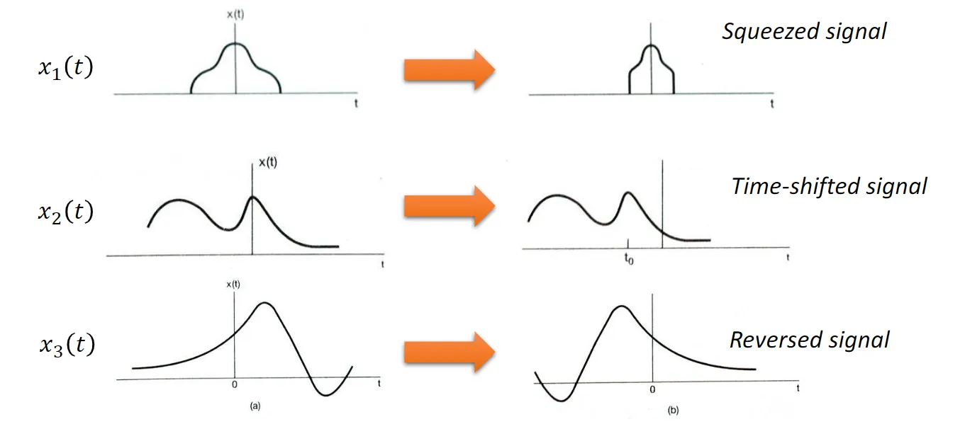
- time scaling x(t) -> x(t/a) (discrete signals often are not "squeezable" though extendable)
- time shift
- time reversal(actually a special form of scaling)
transformation of discrete signals in the y-axis
(for continous ones just refer to calculus) Fisrt difference: y[n] = x[n] - x[n-1] DT Unit Step Signal -> first difference/Pointwise subtraction-> DT Unit Impulse Signal Running sum of a DT signal: If you first take finite dif, and then the running sum, we don‘t get the same signal(+C)
C(continous)T(time) sinusoidal signals
A sinusoidal signal that is derived from a standard cosine function through time scaling/shifting.etc
properties
- periodicity: x(t) equals itself after a time shift of T0
- a time shift is equivalent to a phase change
- symmetry of sinusoidal signals
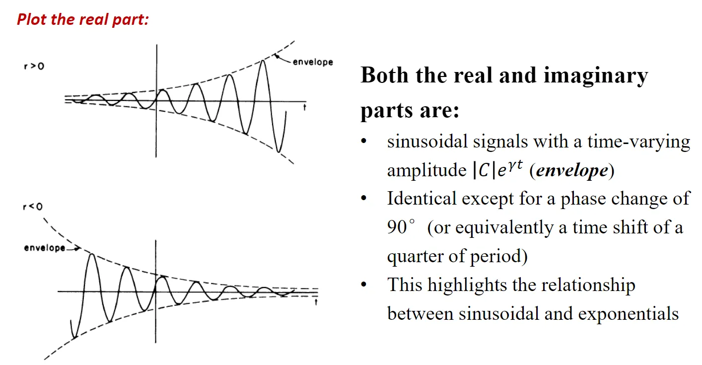
CT complex exponential signal
Algebraic definition: let , and we get
The rectangular/Cartesian form of complex exponential signal
Signal decomposition
almost all real signals can be represented by linear combinations of sinusoidal signals. almost all complex signals can be represented by linear combinations of complex exponential signals.
D(discrete)T(time) complex sinusoidal signal
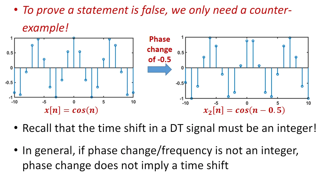
(lost) properties
- phase change != time shift(reverse holds)
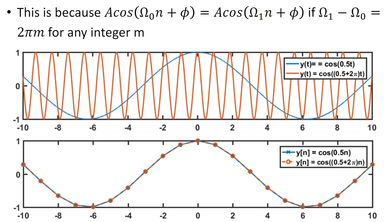
- not neccessarily periodic(only when )
- different frequencies may not imply different signals
DT real exponential
Algebraic definition: can only be seen as the direct sampling of CT real exponential () when
DT complex exponential
Algebraic definition: Rectangular form: it is a direct sampling of CT complex exponential signals
Energy and power of signals
energy:
power
where | | means absolute value for real and magnitude for complex
Unit step & unit impulse
DT
step: u[n] = 1 if n>=0 else 0 impulse: u[n] = 1 if n==0 else 0 unit impulse is the first dif of the unit step, unit step is the running sum of unit impulse
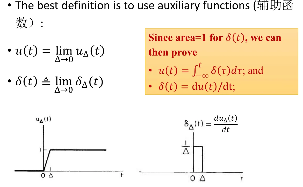
CT
it will be ill-defined if we just copy the discrete definitions into the continous field.
Further Introduction to Systems
Equations for descriptions of systems
systems are not normal functions...or to be more precise, they take a function as a variable, and output another...
- Time-shifting sys:
- Time-scaling sys:
- Squarer:
- Differentiator:
- Integrator:
System interconnections
- Series interconnection/cascaded interconnection: order (generally) matters
- Parallel interconnection: order does not matter
- Feedback interconnectoin: order matters
Systems properties
System properties are partial knowledge about the input/output relationship: Memoryless, Causality, Invertibility, Stability, Linearity, Time-invariance(The first two are time-dependent and the rest are not)
- Time-dependent properties: it only considers how systems behave along the time dimension
- Time-independent properties: it only considers how systems behave along the signal dimension(about matching one input into another)
Properties
- Memoryless property:
- it only depends on the current time point
- Causality property:
- it only depends on previous knowledge
- second order DT differentiator(y[n] = x[n-1] + x[n+1] - 2x[n]) is not causality
- Invertibility:
- there is only one input signal for every output signal
- Running integral have invertibility
- Stability:
- if a small input generates a small output(bounded input generates bounded output, or BIBO)
- if x(t) is bounded , there is a positve m that |x(t)| < m for all t
- squarers are stable
- A running integral/sum is not stable(note that the bound doesn't apply to t, but to x(t))
Convolution
Convolution only exists on linear and time-invariant systems, it mathematically describes how to predict the output for linear and time-invariant systems, it can be implemented by both hand calculation and computers.
- Linearity: defination
- x1 -> y1, x2 -> y2, then x1 + x2 = y1 + y2
- ax1(t) -> ay1(t) for any complex number a
- (a combined version) a1x1 + a2x2 -> a1y1 + a2y2
Systems with the form , where represents a linear system, and represents a signal independent of , are called \textit{incrementally linear systems} (to indicate they are linear systems except for addition of another fixed signal), where y0 is known as the zero-input response
- Time-invariance: aka "shift-invariance"
- x(t - t0) -> y(t - t0) (similar with DT ones)
- (a sum of weighted, shifted unit impulses)
Convolution sum&integral
DT LTI systems Let represent the unit impulse response: . for any LTI:
Apply this property to
we have:
however, this wont work with CT systems, for CT it is:
we see the change is that it is not just the response times the pulse(since the pulse is infinity, we times an additional d, which I suppose can be understood as... the duration?
for DT it is conv sum, and for CT it is intergral, but most of the time we just call it convolution in general.
Some properties
Mathematical Properties:
- x[n] * h[n] = h[n] * x[n] (commutative property)
- x * {h1 * h2} = {x * h1} * h2 (associative property) Above makes two cascading LTI systems switchable
- if x(t) -> y(t) then dx(t)/dt -> dy(t)/t (differentiation property) It allow syou to predict the output of a signal(e.a if you know the response of a step signal you know what the response of the impulse signal is like)
Implementation of convolution
RSMS/RSMI procedure
- Reverse , generating
- Shift the signal by , generating
- Multiply with , generating
- Sum from to , generating for CT signals it's basically the same, except the last step is integral instead of sum
Use of convolution
Convolution can be used to prove some properties of a system in a more straightforward way
Memoryless?
-
Given a system is LTI, the system is also memoryless iff
which is equivalent to say only if , that is, only if .
-
Without loss of generality, only if means:
Since , the only memoryless LTI system is the rescaling system.
Causality?
-
General definition: For any , its output , and any time index , is dependent only on for
-
Given a system is LTI, the above condition means
depends only on for
-
That is, for . That is, for
-
In other words, an LTI system is causal if
Note this is much easier to evaluate than the original definition of causality!
"Initial Zero"
An initial-rest system generates nonzero output values only after the input signal becomes nonzero.
a causal or a memoryless system doesn't necessarily have the initial rest property. But a LTI system have causality if it has initial rest, the reverse also applies.
Stability?
-
Recall the definition of stability: bounded input generates bounded output (BIBO)
-
Assuming LTI, BIBO holds if and only if the impulse response is absolutely summable (integrable) (integration/sum not infinity)
Invertibility?
-
Recall the definition of invertibility: a system A is invertible if and only if different inputs always generate different outputs.
-
When A is invertible, there exists another system A₁, such that the cascaded system (A- A₁) is an identity system.
LCCDE Systems
Linear Constant-Coefficient Differential Equations Systems.
From LCCDE to LCCDE systems
The order of LCCDE refers to the highest derivative of the output y(t) (that is, N).
solving it: homogeneous solution + particular solution
LCCDE have infinite solutions, but LCCDE systems don't, because LCCDE systems have initial state
We can manully select a time, and make it the starting point, this starting point might not have a zero response, and the response the moment before the starting point are seen as the initial state.
LTI and LCCDE systems
Zero-state response: response of the system when there is no initial state = response of the system to the input signal
Zero-input response: response of the system when there is no input = response of the system to the initial state
Solving LCCDE Equations
Solving the solution directly
Solve a 1st order LCCDE:
Particular solution of this LCCDE strictly satisfies the equation.
- A general form of solution to is
- Plugging in the values, we get .
- Solving for K, we find .
- Thus, the particular solution is: .
Homogeneous solution is the function satisfying .
-
Homogeneous solutions are of the form .
-
Substituting into the homogeneous equation gives . Thus, and is the homogeneous solution.
-
Note that can be any number, and the homogeneous equation will still be satisfied.
-
There is an infinite number of homogeneous solutions, each in the form for some number .
-
The complete solution to the LCCDE is the sum of the particular and homogeneous solutions: .
for this example, that is: .
- Every LCCDE has infinitely many solutions, each expressible by a sum of the particular solution and one homogeneous solution.
Classical Approach
Wiped out the u(t) and assume it is only in the positive time domain(which is often the case in real life) and solve it in the (I suppose is more like the) normal and intentional way
Take the previous example:
-
Modify the equation to , . [ dropped & added]
-
The particular solution for the modified input must be of the form . That leads to (Instead of for the original equation)
-
The homogeneous solution is still . is to be determined by the initial state.
-
The complete solution for the modified input is thus , [Initial state is NOT directly applicable].
-
Then, we need to use the continuity assumption about the system output, that is, the output signal is a continuous function at any time (true for most realistic systems).
-
By the continuity assumption, . Then .
-
Thus, the homogeneous solution for the classical approach is (Instead of for the original equation)
-
The total output is then for . (the total output is equal to that derived from the original equation)
| The classical approach | Solving the original equation |
|---|---|
| - is the particular solution (forced response). | - is the particular solution (zero-state response). |
| - is the homogeneous solution (natural response). | - is the homogeneous solution (zero-input response). |
| Par. and hom. solutions DO NOT correspond to zero-state and zero-input response | Par. and hom. solutions correspond to zero-state and zero-input response |
Fourier Series Representation of Periodic Signals
Before we are using impulses as the building block to represent signals (especially in convolution), but the properties of the impulse make it quite complicated to represent some signals, for example, for with impulse it can be represented as with complex exponentials it is which obviously looks better than the impulse solution
HRCE(Harmonically Related Complex Exponentials)
A set of signals, , is called a set of Harmonically Related Complex Exponentials if and only if
Where is called the fundamental frequency for the set of harmonically related complex exponentials.
- Harmonically Related Complex Exponentials (HRCE) is a set of complex exponential signals.
- These exponential signals are "harmonically related", in that the frequency of is (-fold multiple of the fundamental frequency).
- A set of HRCE is known iff its fundamental frequency is known.
- can be both positive or negative integers.
- they share a common period(T0)
The Fourier Series Representation
- is called the Fourier series coefficient or the spectral coefficient of .
- is called the Fourier series spectrum of .
- Equation (1) is called the synthesis equation: almost every periodic signal can be synthesized/represented by a linear combination of harmonics in the HRCE.
- Equation (2) is called the analysis equation (spectral analysis): it tells you how to generate the coefficients for the FS representation.
We also have the "Partial Sum":
It's easy to recognize that
Displaying The FS Spectrum
- When we have the Fourier series spectrum, we often want to plot the spectrum, because it reflects the frequency components contained in .
- However, notice the Fourier series coefficients are complex numbers, so we need at least two plots to show the spectrum (magnitude & phase).
For example: let's display the FS Spectrum of the following signal
Collecting terms, we obtain
Thus, the Fourier series coefficients for this example are
to polar form
and we will get two plots:
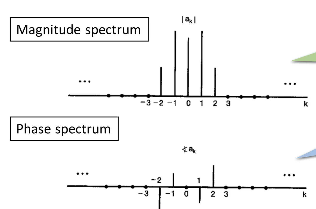 both parts are critical for describing a signal, if a signal has shifted in the time domain, the magnitude spectrum will very likely to remain unchanged while the phase spectrum will have changes(and it's not simply a shift in the whole pattern)
Spectrum Analysis for LTI Systems
Eigenfunction
Definition: for a given LTI system, an input signal that generates an output signal that is simply the input multiplied with a constant is called an eigenfunction of the system.
If , then is an eigenfunction of the system , and is the eigenvalue associated with the eigenfunction. (quite similar for definition for the eigen-things in linear algebra)
complex exponentials are always eigenfunctions of an LTI system.
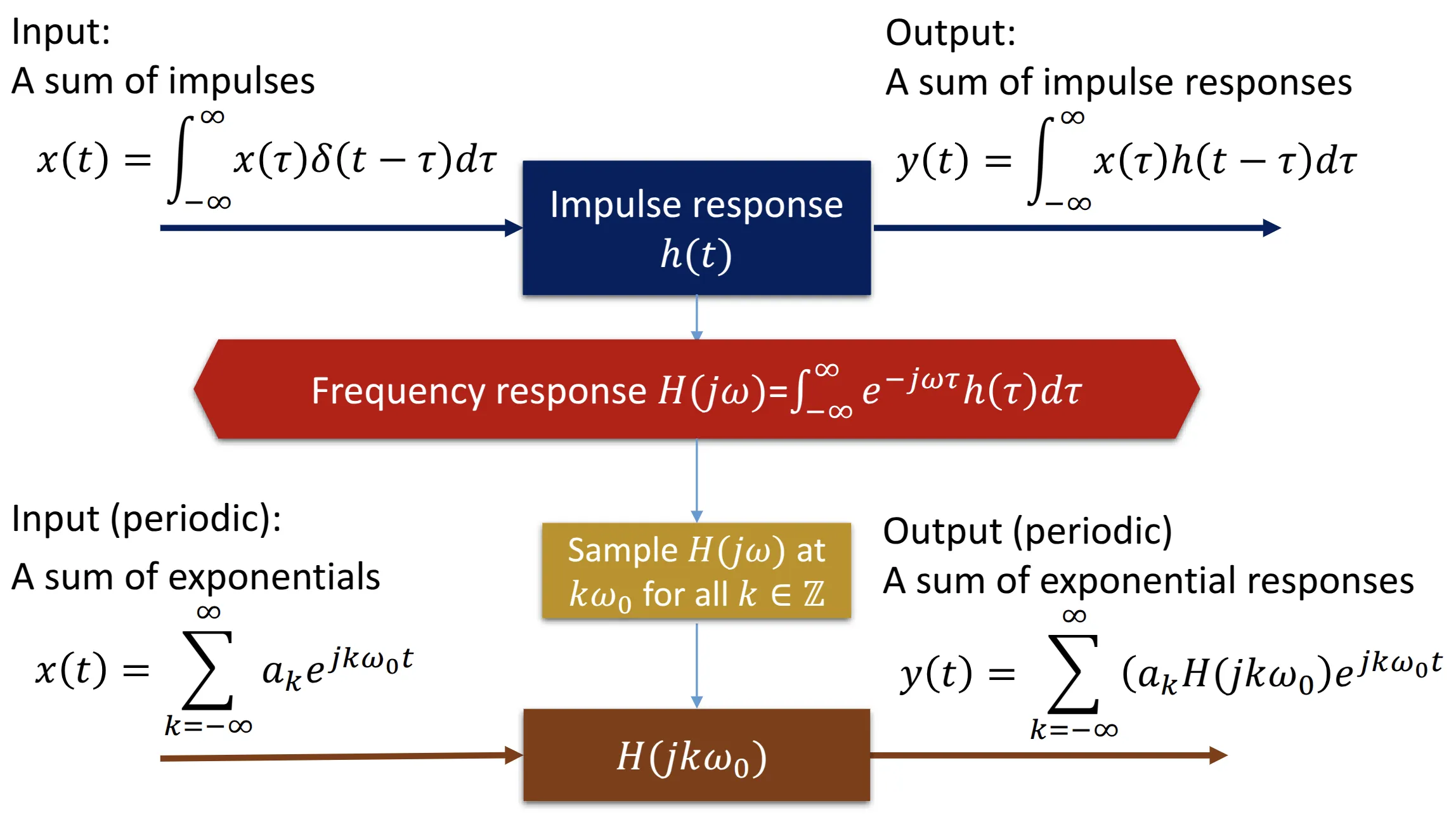
A New Way of Analyzing LTI Systems
Let , then the output is
Since is not dependent on , we can write the output as Where The eigenvalue associated with . It is dependent on the frequency , the impulse response, but not on .
Fourier series representation decomposes a signal into a linear combination of harmonically related eigenfunction signals.
Then the response of an LTI system to an arbitrary periodic signal would be Output is a periodic signal with the same period & a spectrum of
Generally the idea is, any input signal can be broken down to a series of eigenfunctions of any LTI system, so the input can be assembled from a series of eigenfunctions, rescaled according to the corresponding eigenvalue.
Advantages
- First, computational advantages over convolution. For example: what is the output for and ?
- Convolution is difficult
- Frequency domain:
- is nonzero only for .
- Note that since , only for
- Second, it provides critical insights to help us understand how the system changes each harmonic:
- If is greater than 1, the harmonic gets strengthened in the output spectrum
- If is less than 1, the harmonic gets attenuated (weakened) in the output spectrum
The second one leads to the important concept of "filtering".
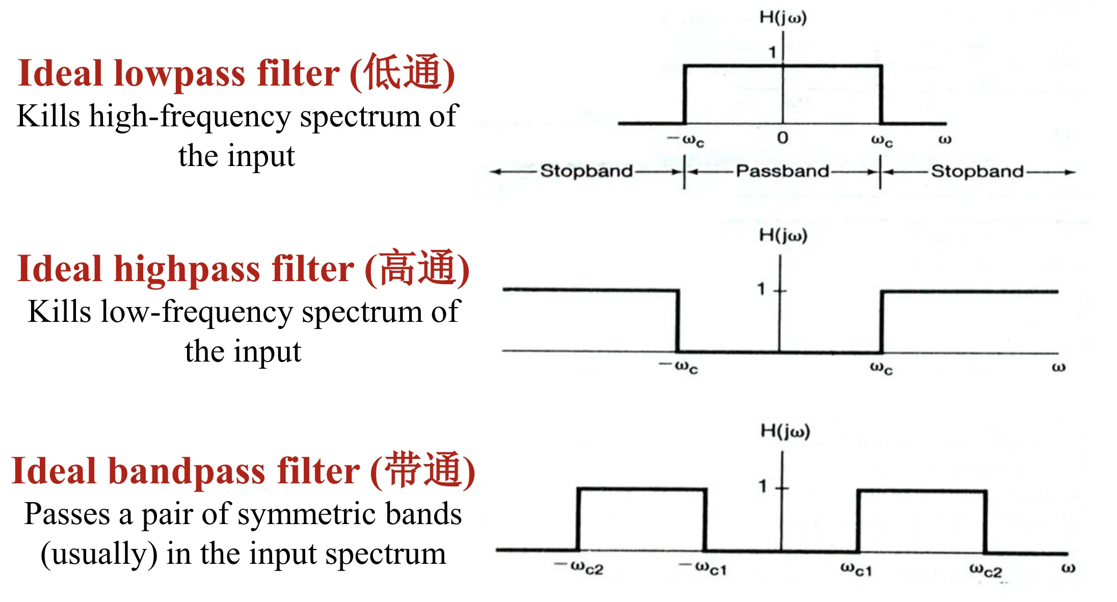
Filters
So the filters is mostly a function for H(j)
-
Type one filters(Frequency-selective filters, or ideal filters): just 1 or 0, no other values
-
Type two filters(requency-shaping filters): most reshape, not completely kill or live
 (actually this is the filter for differentiater)
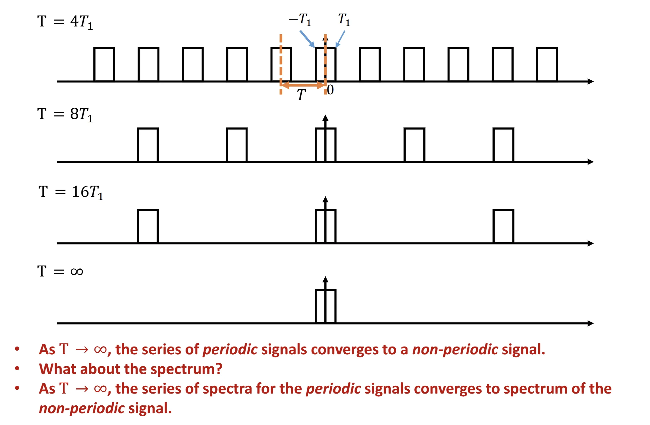
Performing Fourier Transform on Aperiodic Functions
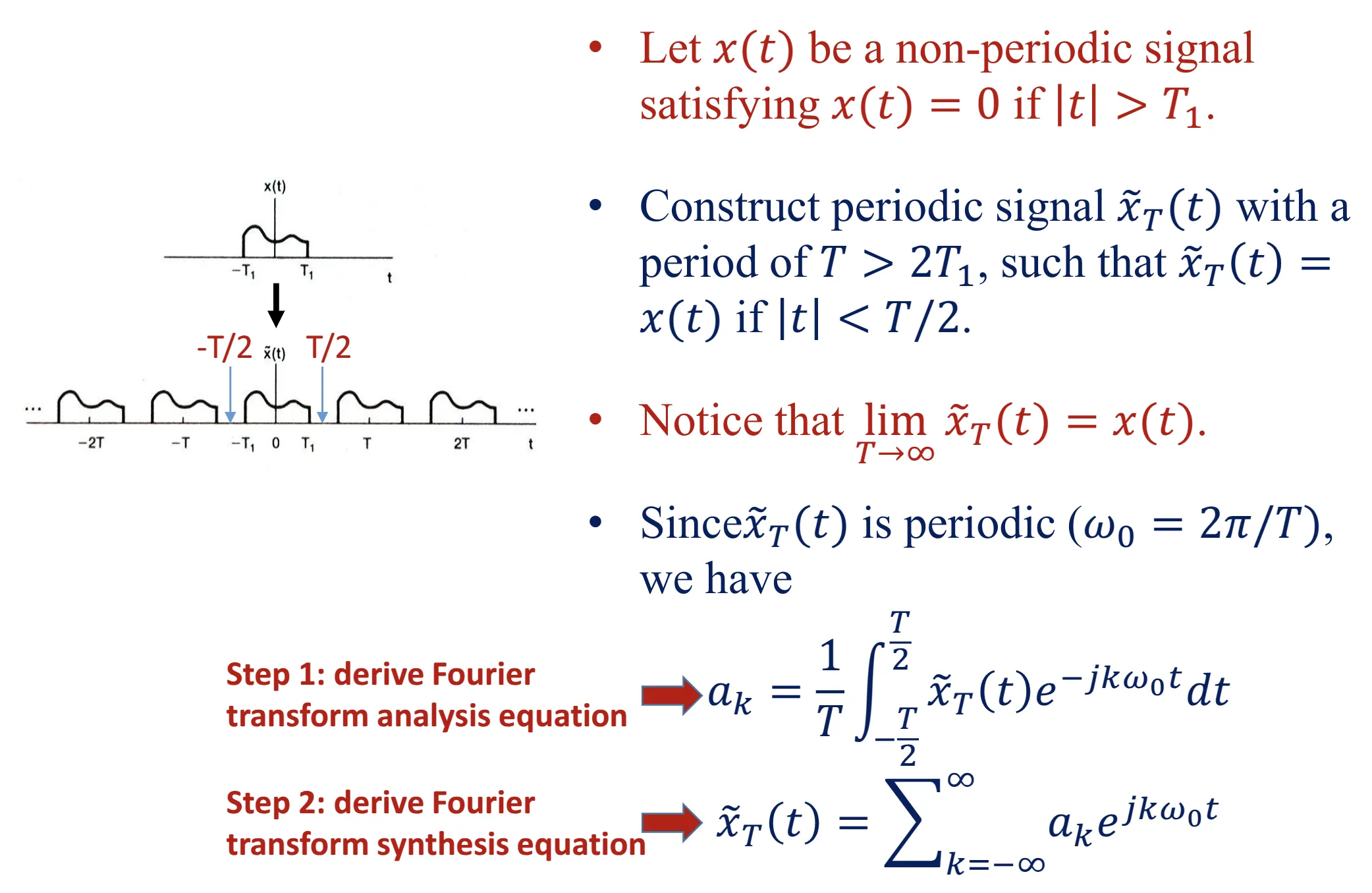
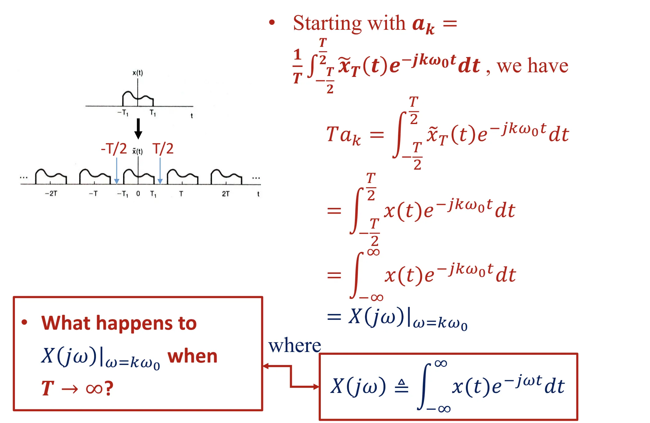
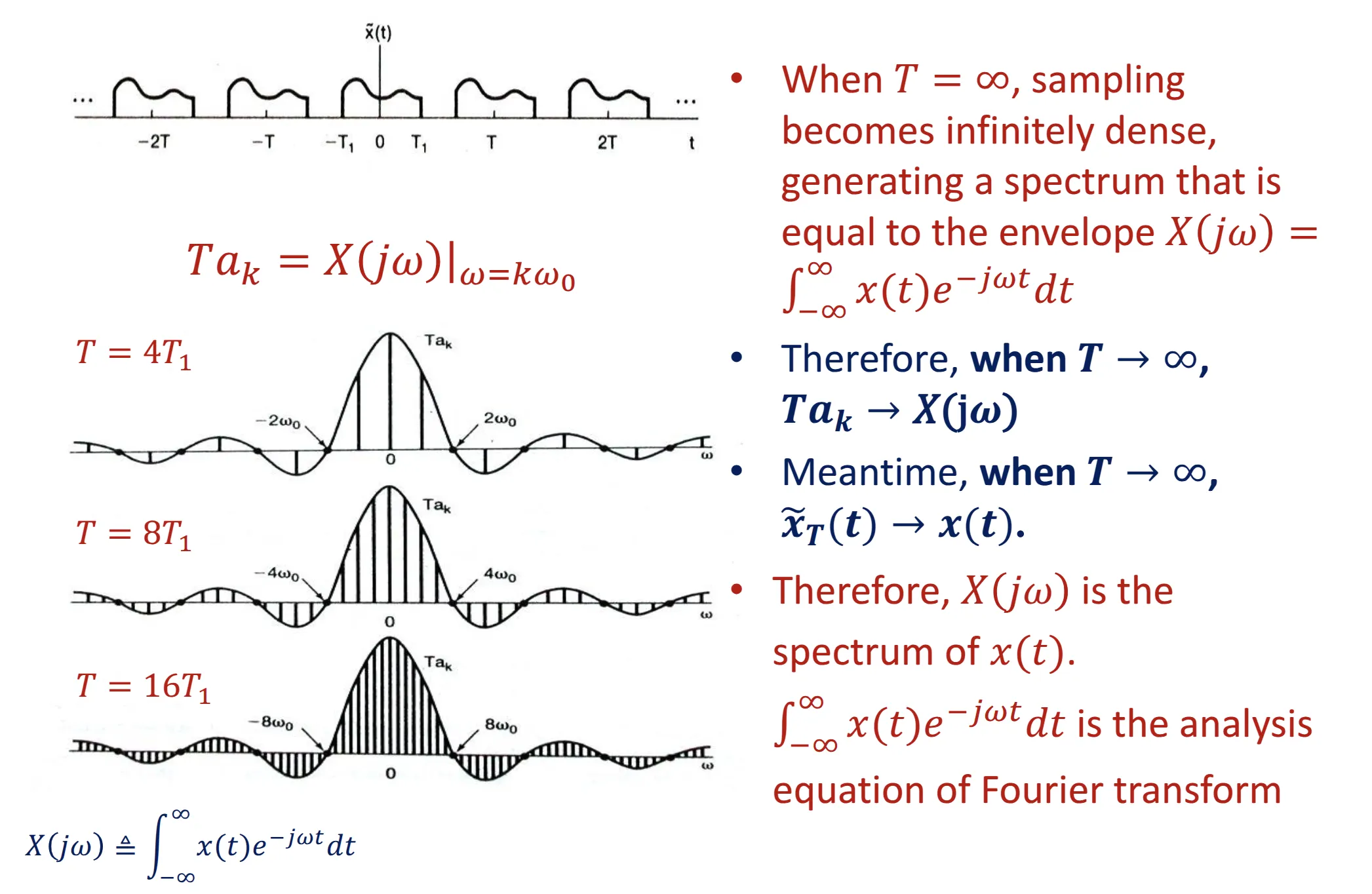
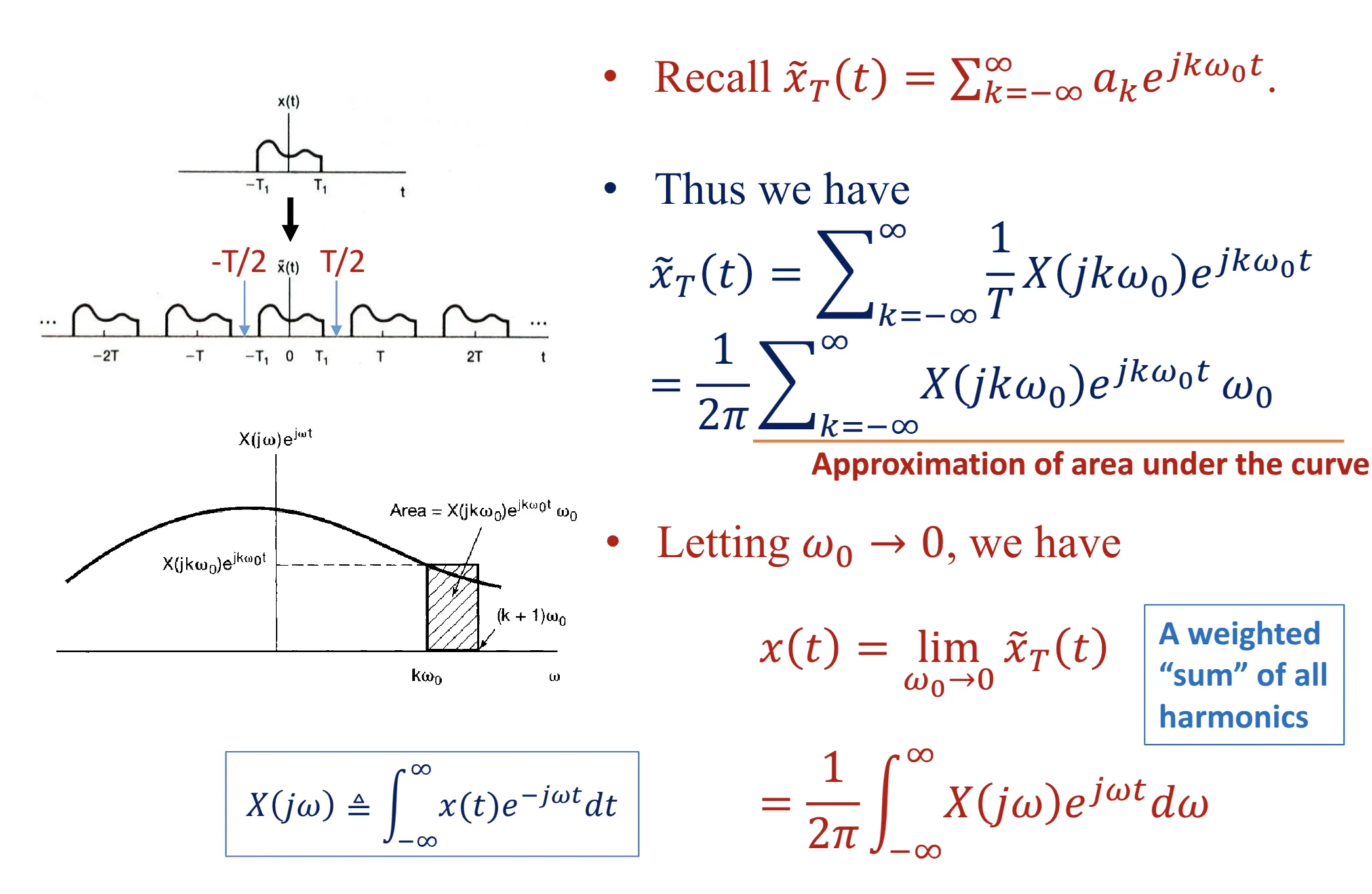
Fourier transform
previously Analysis Equation
Inverse Fourier transform
previously Synthesis Equation
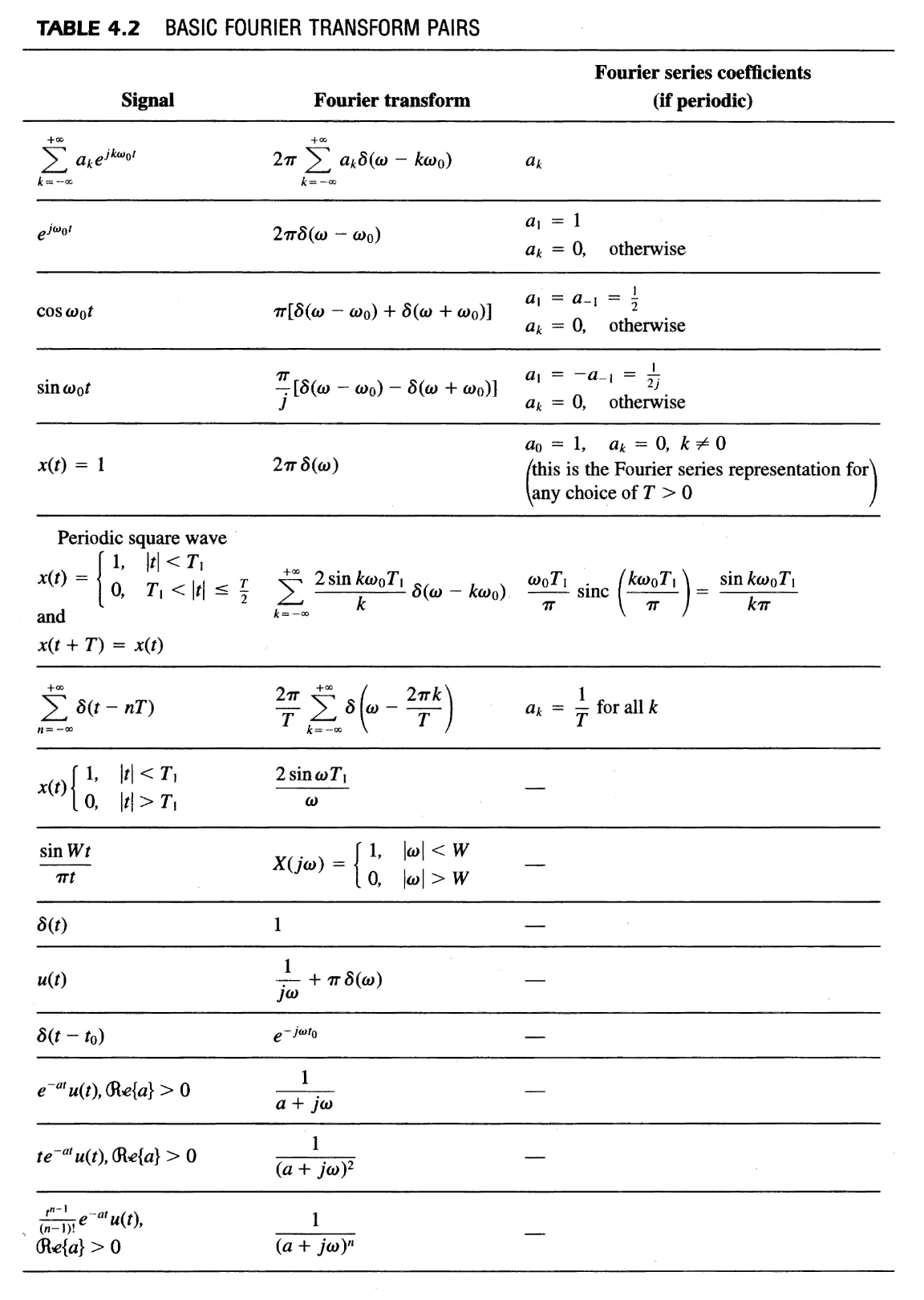
Fourier Transform Pair
If , we say and are a Fourier transform pair.
A well-known Fourier transform pair is the rectangle-sinc pair, that is, the Fourier transform of a rectangle signal is a "sinc" signal.
This pair is very important because we often need to analyze the FT of a rectangular signal or IFT of a rectangular spectrum.
Fourier transform pairs are completely invertible, for example, a "sinc" in time domain will be a "rectangle signal" when transformed to the frequency domain.
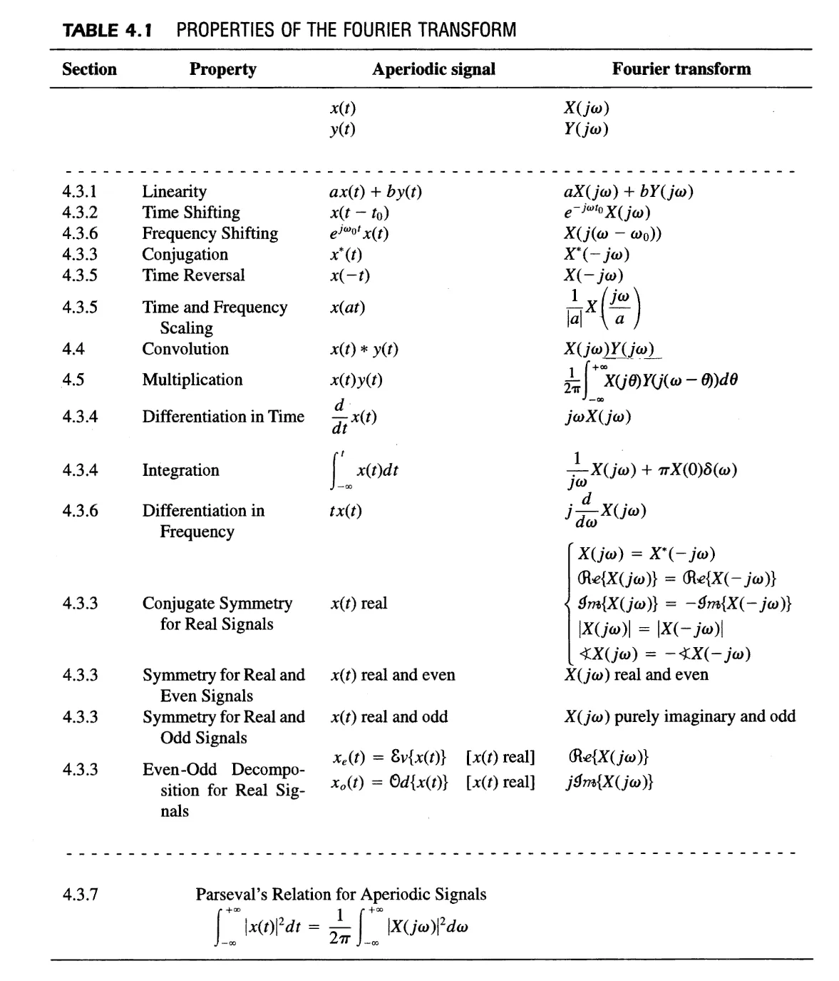
Properties of Fourier Transform
Performing Fourier Transform on Periodic Signals
To find the Fourier Transform (F.T.) spectrum of a periodic signal , we are looking for a spectrum that satisfies:
Let be the Fourier Series (F.S.) spectrum of . If Equation (2) holds, we must have:
The left side is a "sum" over all frequencies, while on the right is sum over a discrete set of frequencies
So X(j) is some function times , and the function is only non-zero on certain frequencies, which is an impulse train.
The equation indicates that is an impulse train located at the harmonic frequencies .
That is The Fourier Transform for Periodic Signals
Linearity
For sure
Time shift
Fourier transform:
which is generally the same with
Fourier series:
Time reversal
Fourier transform:
which is still generally the same with
Fourier series:
Two indications(Also works with fourier series):
- If is even, then is even, and vice versa.
- If is odd, then is odd, and vice versa.
Conjugacy & Symmetry
- Fourier transform:
which is also the same with
-
Fourier series:
-
subcases
-
If is real, "conjugate symmetric". => Real part is even, and imaginary part is odd.
-
if is real and even, is real and even
-
if is real and odd, is imaginary and odd.
-
A new indication not mentioned before:
- Since a real signal , real spectrum + imaginary spectrum.
- Meanwhile we also have . This means:
-
below here the properties that start to change
Differentiation and Integration
-
Differentiation property of Fourier transform:
-
The same as for the Fourier series: If , then
-
Indication: differentiator is a highpass filter (non-ideal)
-
-
Integration (Different!)
-
If , then
-
Fourier series: Suppose , and , then
-
Why this happens?
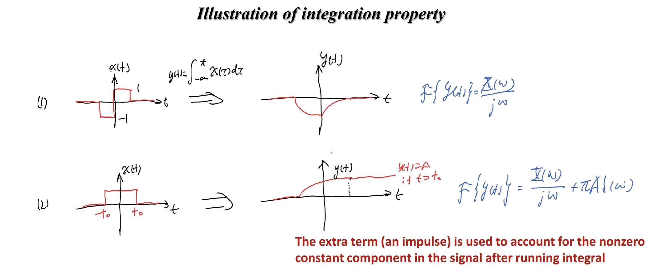 so this is actually the same with the fourier series, but in series we can explicitly say = 0, but this is often not the case for fourier transform, so we have to add this term, which is actually the area under the curve.
-
Parseval's Theorem
-
Fourier transform
- If then
- If then
-
Fourier series
- Suppose
then
- Suppose
Time scaling
-
If , then for any and .
- If , is squeezed to generate , is stretched and downward scaled to generate .
- If , is stretched to generate , is squeezed and upward scaled to generate .
-
The scaling of the signal is opposite to the scaling of the spectrum.
- Squeezing of signal causes faster variation, thus more high frequency components.
- Stretching of signal causes slower variation, thus more low frequency components.
-
E.g. , where
Duality
If , then , or
Convolution
recall this
now we find that this so-called frequency response is the Fourier Transform of the impulse responce, from we can derive the convolution property:
proof:
Multipication
which is actually the duality of the convolution propertyy
Predicting Outputs of a More Specific Systems
(This part is mainly based on the convolution property)
Interconnected Systems
for two systems that has the frequency response of and
Cascaded Systems
very easy,
Parallel Systems
still easy,
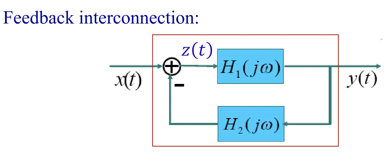
Feedback Systems
where things get compilcated, take below as an example
LCCDE Systems
For the LTI subsystem of a stable LCCDE system
Example: Find impulse response of
Assuming the system is stable
Time-Frequency Analysis of LTI/LCCDE Systems
The Impact of Spectrums and Phases
The spectrum, or |H(j )|, officially known as the gain of the system, changes the input spectrum by multiplication.
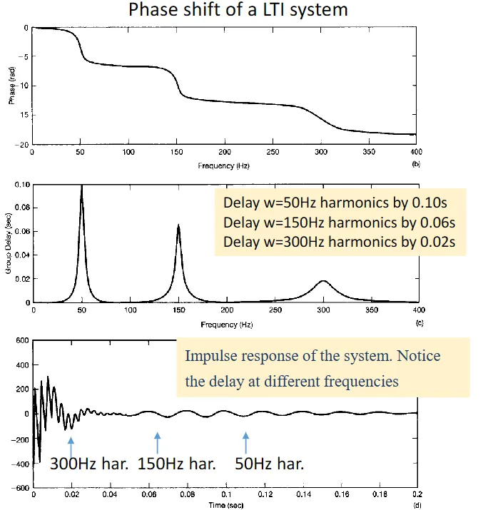
, formally called phase shift of the system, affects the phase of the input spectrum by addition.
So we know that, if the phase is linear, it will delay the signal, which is something don't want.
And there is something we don't want more: if the phase is non-linear, then the delay for different frequencies will be different, causing distortions and errors.
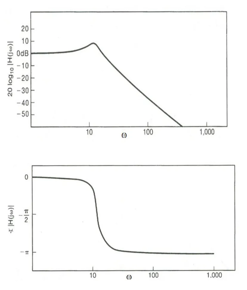
The Bode Plot
While the sepctrums/phases plots we drawn before seems good and straight forward, it is not used a lot in practice, where the filters might encounter frequencies at a very wide range, and the spectrum might also change in a very wide range, and the linear X, Y axis is not enough anymore, so we introduce the bode plot. It's still plots with frequencies as X-axis and spectrum/phase as the Y-axis, but instead of linear, it's log.
Bode Plot
The X-axis of a bode plot is in a log scale, that is the first tick is a, and the next tick is 10a, next 100a, 1000a and so on, an increase of 10 fold is called a decade. The Y-axis is in a 20log10 scale, and one unit in this scale is called a db, so the slope is described as xxdb/decade.
A very good thing of the spectrum bode plot is that it transforms the multiplication to addition, now, we just need to add the signal bode plot with the filter bode plot to get the result bode plot, much easier the multiplication.
And for the bode plot of phase, while the Y-axis keeps it's original phase, the X is in a log scale, like the spectrum bode plot.
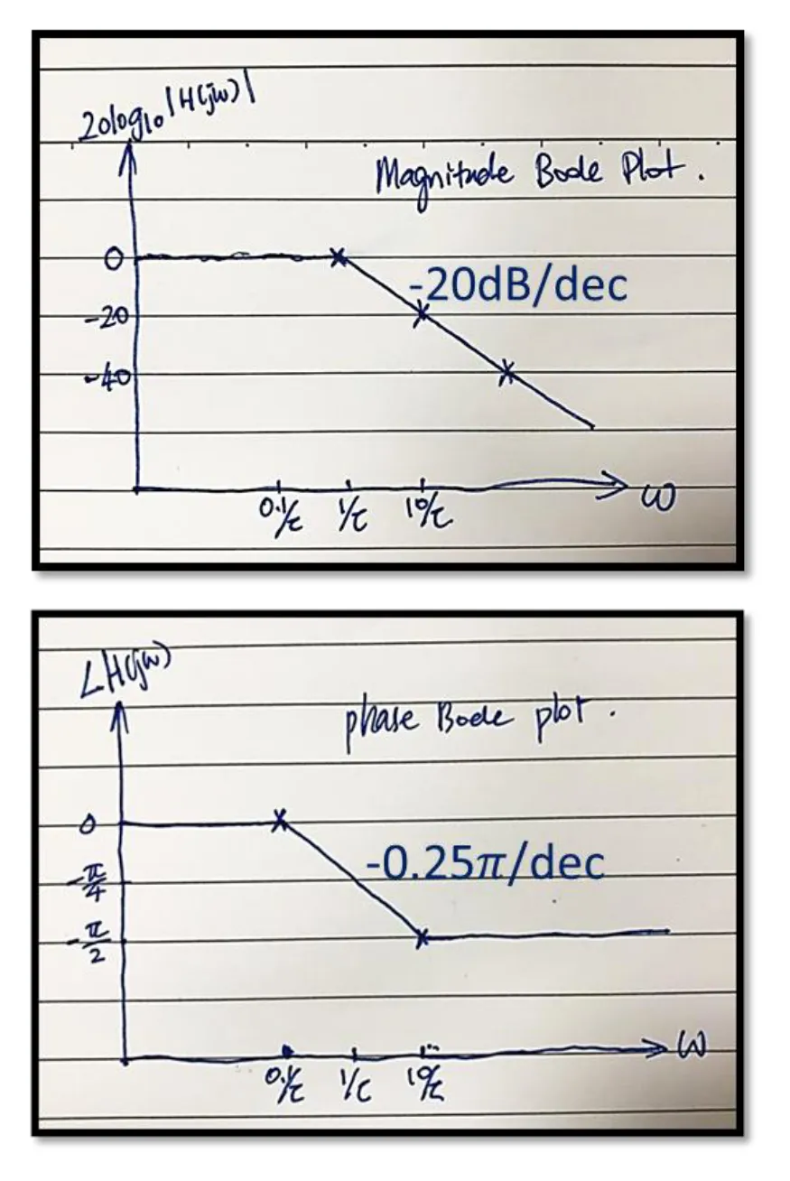
Asymptotic Bode Plots
Unfortunately the exact bode plot, like the ripples on the turning points, are not easy to plot. So we introduce the asymptotic bode plots, it focuses more on the trend and not the details, for example:
- Spectrum:
- When ,
- When , , which is a straight line with a slope of -20dB/dec and a value of
- Phase:
- When ,
- When ,
- When ,
so it looks like
How to Draw Asymptotic Bode Polts
(唉懒得装模做样说洋文了这段我就用中文说吧)
反正就是要拆成常数项和, 然后分子上的每一个会从开始给振幅图提供+20db/decade的斜率,给相位图从提供/decade的斜率(如果有平方项就算两次以此类推)
分母上就都是负的
然后常数项若为K,在振幅上决定纵轴截距为,在相位上就是正数的话无影响负数的话纵轴截距为
Sample Theory
Signal to Sample
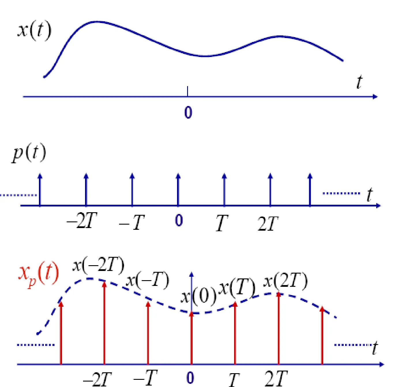
Where T is the sampling period, then
where p(t) is called the sampling function, and 2/T is called the sampling rate.
Sampled Signals Analysis
first we can discuss about the specturm of the sampled signal, from the multiplication property we know that the spectrum of the signal:
so, the sampled signal is a series of original shifted spectrum added up together.
Now, for simplicity, we assume that the original signal is banded-limited (from to ), the sample spectrum are the original spectrum, and move it to left or right, and add it to the spectrum and so on.
If we are lucky, the gap is wide enough so there is no overlap, we will have a "spectrum" train, and we just apply a low pass filter to get one, and ift it to get the very original signal back.
But there are times we are not so lucky, where the gap is not that wide and there is an overlap, then spectrums start distorting each other, and now there is no way to recover it perfectly.
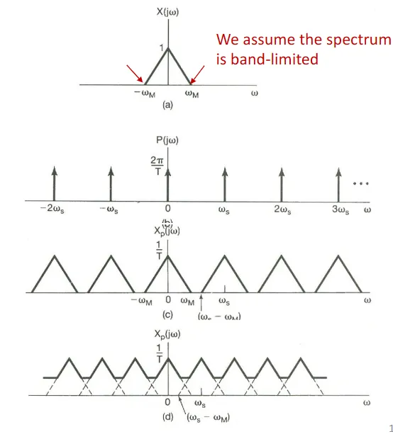
So we quantify the "gap" here and we get the Nyquist-Shannon Sampling Theorem:
Let be any band-limited signal with for . Let be a series of its periodic samples with a sampling frequency of . If and only if , can be uniquely determined by its samples through the following process:
- Generate the impulse-train sampled signal:
- Apply an ideal lowpass filter with a gain of and a cutoff frequency . The output of the lowpass filter is
ZOH sampling
In practice, we don't use impulses that often, we use a sort of sampling type called, zero-on-hold, aka sample-on-hold. Generally, instead of just having an impulse on the sample point, it will keep the value, until the next sample point, making a stair like sample result.
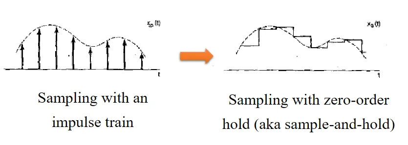
will this seems like a small change, it's not that beautiful in the frequency domain. First, we need to know that this is mathematically the impulse sample convolves with h(t), where , and the spectrum for h(t) is , a nasty one!
so for this we have
and we want
where X_p is the impulse sample result, and H(j ) is a low pass filter (cutoff at / 2 for example)
from above we can see that we can use s "inverse filter" for H_0, which is possible:
Aliasing
I can only explain it in an intuitive way. Let's consider the expected sampled spectrum as a 'true' specturm, and it's shifted mirrors, why we sample on a low frequency? Not because we want to get the low-pass part, what we really want to get is the 'true' part. And aliasing happens when the 'true' part actually is out of the filter range, but a 'fake' shifted mirror is captured in the sample range.
or just see 13:16-15:13 of this video
Aliasing happens to a harmonic when the frequency of the harmonic is greater than . And the practical solution is to just cut off all the harmonics higher than half the sample rate before sampling.
Digital to Analog
Digital signals are mostly discrete, and analog are mostly continuous, so we need to interpolate some data points into the digital signals' gaps before converting
Given a set of samples , interpolation refers to where is referred to as the interpolation basis
here we briefly introduces three types of interpolations:
- sinc interpolation: convolve the impulse sample with sinc function.
- PROS: that's the perfect rebuilt theoretically, as sinc function is a low pass filter in the spectrum domain, and thats the very filter we want mentioned above.
- CONS: convolution means you have to rebuild on the whole time scale, which is almost impossible in real life applications, this way of interpolation is only of theoretical significance.
- zero-order interpolations: pretty much like the reverse of ZOH sampling, the interpolation basis is like the h(t) above.
- first-order interpolations: connect discreate dots with a straight line, the interpolation basis is a trianglar funciton.
Laplace Transform
Fourier is great...in most conditions, but there is a problem with the 1st Dirichlet condition, the signal must be absolutely integratable, which is not the case for all the signals/systems. Therefore we introduce the Lapalace Transform, which is actually like fourier transform expanded.
For an arbitrary signal ,
is referred to as the Laplace transform of , where is a complex variable.
Fourier transform is a special case of Laplace transform when (i.e., on axis in -plane)
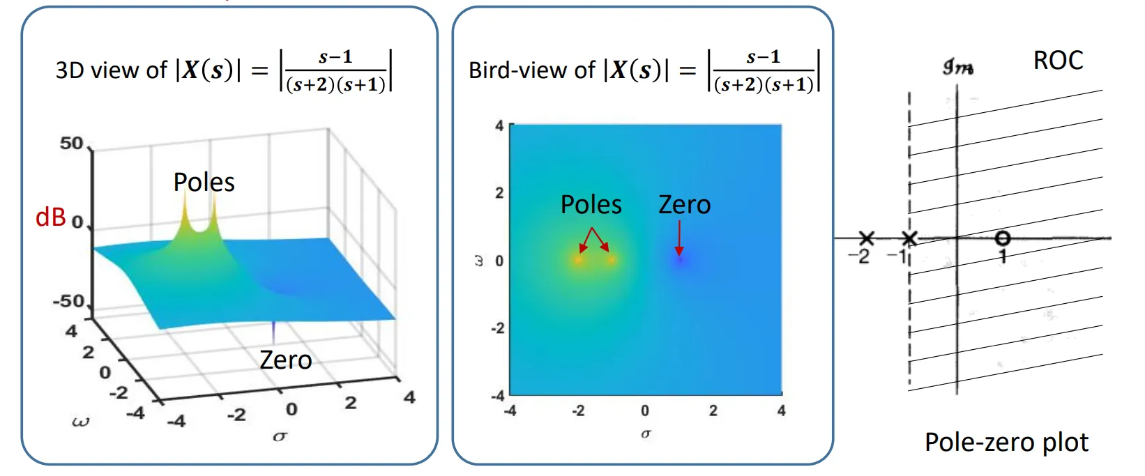
ROC
(这后面是我暑假期间补写的, 所以我也不想演了, 用中文吧) 正如我们之前所提, 傅里叶变换的最大的问题就是对很多信号或者系统用不了, 所以我们引入了拉普拉斯变换, 其本质就是给函数补了一项 , 让他本来可以不能用傅里叶了可以傅里叶了, 所以从图的角度来看本来傅里叶变换就是一条线变成了另一条线, 但是由于拉普拉斯加的这项额外引入了一个变量 所以就从一条线可以变换成很多(方向平行)的线, 组成了一个二维的面. 当然, 并不是所有的 都能让信号收敛, 能使其收敛的这部分的 取值就叫做收敛域(ROC, region of convergence)
零极点图(Pole-zero plot)
如果我们想可视化拉普拉斯变换的光谱, 按照傅里叶变换的画法, 我们需要画一个凹凸不平的曲面, 虽然对电脑没问题, 但如果想手绘的话显然需要一些画工. 显然大部分时候我们都不需要所有 对应的拉普拉斯变换后的频谱, 我们可能更关心特殊情况, 比如什么时候是零点, 极值点, 这就可以用零极点图来表示, 也就是把所有的 取值画在一个平面上, 然后把对应的 的零点和极点标出来. 按照惯例我们把零点用圈圈, 极点用叉叉标s平面上标出来, 再用虚线和阴影标出可行域.
ROC的性质
-
ROC的边界一定垂直于s平面的横轴(实轴), 即ROC一定是一个或者数个相互平行的竖直带状区域.
这是因为 是个实数
-
ROC不包含极点
ROC是收敛域, 而显然, 极点并不收敛
-
如果x(t)非零区间有上下限内非零或绝对可积, 则收敛域是整个s平面
即证 时, .
即
-
如果x(t)非零区间有下限, 则若 收敛, 则 也收敛
即ROC是一个右半平面
-
如果x(t)非零区间有上限, 则若 收敛, 则 也收敛
性质4的镜像版
-
如果拉普拉斯变换后的结果为有理函数, 则其ROC的边界要么为极点, 要么无限
-
如果x(t)的拉普拉斯变换后结果有理且存在ROC, 那么其满足:
- 若x(t)右半边非零, 则其收敛域左边界为最右侧极点, 右边界为无限
- 若x(t)左半边非零, 则其收敛域右边界为最左侧极点, 左边界为无限
- 若x(t)双边非零, 则其收敛域左右边界分别为两相邻极点
拉普拉斯逆变换
回顾拉普拉斯变换:
由于我们之前提到过, 拉普拉斯变换的本质是把原函数偏移了一下的傅里叶变换, 即
因此我们可以得到拉普拉斯逆变换为:
计算拉普拉斯逆变换
硬算由于涉及含复数的积分, 比较困难, 对有理的拉普拉斯变换通常我们可以拆成一些已知的拉普拉斯变换对来进行逆变换的计算. 常见的包括
| Transform pair | Signal | Transform | ROC |
|---|---|---|---|
| 1 | All | ||
| 2 | |||
| 3 | |||
| 4 | |||
| 5 | |||
| 6 | |||
| 7 |
需要注意的就是即使变换后的结果相同, ROC不同, 原信号也可能完全不同.
拉普拉斯变换的性质
-
线性
, ROC: , , ROC: 时, 有
, ROC 包含(不一定相等) , 例如, 可能ROC的边界是两个极点, 而这两个节点可能一正一副负刚好抵消, 这里这个边界就消除了, 让ROC扩大.
-
时移
, ROC 不变
-
频移
ROC: ROC:
-
时域尺度变换
, ROC:
-
共轭对称性
, ROC: , ROC:
由这个性质我们可以得到, 对于一个实信号, 其的零点和极点要么在横轴上, 要么关于横轴对称
-
卷积性质
, ROC : , , ROC : => ROC 包含
当两个变换的极点和零点重合时, 可能会导致ROC的拓展
-
时域微分
, ROC 包含原收敛域(当其在s=0处有一阶极点时ROC会扩大)
-
s域微分
, ROC: , , ROC:
-
时域积分
, ROC: 包含 (当且仅当X(s)在s=0处有零点时为包含)
-
初值与终值定理
x(t)在t<0时恒为0且x(t)没有脉冲或更高阶奇点时满足
- 初值定理:
- 终值定理: (x(t)在t->∞时收敛)
用拉普拉斯变换分析LTI系统
传递函数
传递函数(aka系统函数)是指一个系统的脉冲响应的拉普拉斯变换, 由于卷积性质, 对任意信号都有 , 因此我们可以用传递函数来预测输.
从拉普拉斯变换视角来分析LTI系统的性质
-
因果性: 若一个LTI系统是因果的, 则其传递函数的ROC是一个右半平面. (对一般LTI倒过来说不成立) 更进一步的, 如果LTI的传递函数是有理(可以表示为两个多项式只比)的, 则倒过来也成立了
-
稳定性: 若一个LTI系统是稳定的, 则其ROC必须包含虚轴, 如果其同时还是因果的, 则说明其传递函数的极点都在左半平面内.